Sales Analysis Project in AI Python Panda Sklearn scikit-learn matplotlib dash core Write up

 

All correct packages like pandas, scikit-learn, matplotlib, seaborn, dash, dash core components and html etc should be installed using pip install

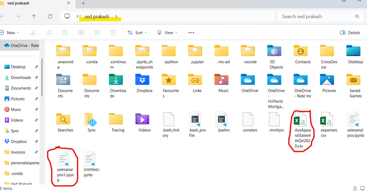
Since this project is going to be saved as a Jupyter notebook file so csv file must be placed in same directory where the notebook .ipynb is saved. Although it can be saved anywhere but if saved same directory then giving filepath would be easy otherwise we have to give path wherever it is needed.

 

If file path will not be given correctly then file not found error will come while executing the code.

Now as per problem statement document, it says first to do data wrangling so

————————————————————————-

import pandas as pd

 

# Load the dataset

file_path = “AusApparalSales4thQrt2020.csv”  # Update with actual file path

df = pd.read_csv(file_path)

 

# Display basic info about the dataset

print(df.info())

 

# Check for missing values

print(df.isna().sum())

 

# Check non-missing values

non_missing = df.notna()

print(non_missing.head())  # Displays True/False for each cell

 

# Count of missing values per column

missing_count = df.isna().sum()

print(missing_count)

 

missing_rows = df[df.isna().any(axis=1)]

print(missing_rows)

—————————————————————————–

Here we are using isna() and notna() function as per problem statement document.

First we import pandas and then load the data set by giving correct file path. If the CSV is in a different directory, you must provide the absolute path. Example:

df = pd.read_csv(“C:/Users/YourUsername/Documents/AusApparalSales4thQrt2020.csv”)  # Windows

df = pd.read_csv(“/home/user/Documents/AusApparalSales4thQrt2020.csv”)  # macOS/Linux

If you’re unsure where the file is, use tkinter to browse and select it:

import pandas as pd

from tkinter import Tk

from tkinter.filedialog import askopenfilename

 

Tk().withdraw()  # Hide root window

file_path = askopenfilename(title=”Select CSV file”)  # Open file dialog

df = pd.read_csv(file_path)  # Read the selected file

 

To see where Python is looking for the file, check the current working directory:

import os

print(os.getcwd())  # Prints the current working directory

If the file is not there, move it to the displayed directory or change the working directory using:

os.chdir(“C:/Users/YourUsername/Documents”)  # Change to the directory where the file is

—————————

With pandas functions of read csv we read csv and store it in df. Then we print basic info of df.

With isna() we check for missing values.

The notna() function returns True for non-missing values and False for missing ones.

This filters rows where at least one column has a missing value.

missing_rows = df[df.isna().any(axis=1)]

print(missing_rows)

Handling Missing and Incorrect Data

• If missing values are minimal (few rows), we can drop them.
• If missing values are in crucial columns, we should fill them using:
  • Mean/median for numerical columns
  • Mode for categorical columns

Recommendation for Handling Missing and Incorrect Data in AAL Sales Analysis

Based on the missing and incorrect data analysis, here are the recommendations:

1️⃣ Handling Missing Data

A) For Numerical Columns (e.g., Sales, Units)

✅ Recommended Action: Fill missing values with the median
📌 Reason:

• Since sales data often has skewed distributions, the median is more robust than the mean.
• Prevents data loss that would occur if we drop rows.

Implementation:

df["Sales"] = df["Sales"].fillna(df["Sales"].median())

df["Units"] =
df["Units"].fillna(df["Units"].median())  # Ensure correct column name

B) For Categorical Columns (e.g., State, Group)

✅ Recommended Action: Fill missing values with the most frequent value (mode)
📌 Reason:

• Ensures consistency in categorical data without introducing bias.

Implementation:

df["State"] =
df["State"].fillna(df["State"].mode()[0])

df["Group"] =
df["Group"].fillna(df["Group"].mode()[0])

C) If Too Many Missing Values Exist

✅ Recommended Action: Drop rows only if missing values exceed 30-40% of total data
📌 Reason:

• If a row is missing too much data, filling may introduce bias.
• If <5% of total data is missing, filling is preferred over dropping.

Implementation:

df.dropna(thresh=int(0.6 * len(df.columns)), inplace=True)

2️⃣ Handling Incorrect Data

A) Identify & Remove Negative Sales Values

✅ Recommended Action: Remove rows where Sales or Units are negative
📌 Reason:

• Sales and units sold cannot be negative.
• These values could be data entry errors.

Implementation:

df = df[df["Sales"] >= 0]

df = df[df["Unit"] >= 0]

B) Fix Spelling Errors in Categorical Columns

✅ Recommended Action: Standardize inconsistent values
📌 Reason:

• Spelling mistakes (e.g., "NSW" vs "New
South Wales") can cause incorrect groupings.

Implementation:

df["State"] = df["State"].replace({"NSW": "New South Wales", "QLD": "Queensland"})  # Example

df["Group"] = df["Group"].str.strip().str.title()  # Fix casing issues

Normalization for Data Consistency

Since sales and units have different scales, Min-Max Normalization is recommended.
✅ Recommended Action: Apply Min-Max Scaling to Sales and Units
📌 Reason:

• Ensures fair comparison across features.

Implementation

from sklearn.preprocessing import MinMaxScaler

 

scaler = MinMaxScaler()

df[[“Sales”, “Unit”]] = scaler.fit_transform(df[[“Sales”, “Unit”]])

Recommendation on GroupBy() Usage

✅ Recommended Action: Use groupby() for sales aggregation by state & age group
📌 Reason:

• Helps in analyzing which states & demographics perform best.

Implementation:

state_sales = df.groupby(“State”)[“Sales”].sum().reset_index()

print(state_sales)

 

group_sales = df.groupby(“Group”)[“Sales”].sum().reset_index()

print(group_sales)

Final Thoughts

By following these data wrangling best practices, AAL will:
✅ Ensure clean, accurate, and usable data for analysis.
✅ Prevent data loss by filling rather than dropping values.
✅ Improve decision-making by ensuring fair comparisons across states and demographics.

 

 

 

Insights on GroupBy() Function for Data Chunking or Merging

The groupby() function in Pandas is a powerful tool for aggregating and analyzing large datasets. It allows us to segment the data based on categories and perform summary statistics efficiently.

1️⃣ Application of GroupBy() for Data Chunking

✅ Why Use It?

• Breaks data into smaller chunks based on categorical variables (e.g., State, Age_Group).
• Helps reduce computational load when working with large datasets.
• Enables parallel processing in large-scale data analysis.

✅ Example: Chunking data by state to analyze total sales per region

state_sales = df.groupby("State")["Sales"].sum().reset_index()

print(state_sales)

📌 Insight:

• This provides a concise summary of sales performance per state, making it easier to identify high and low revenue states.
• Can be used to focus marketing efforts on weaker-performing states.

2️⃣ Application of GroupBy() for Data Merging

✅ Why Use It?

• Aggregates similar data before merging with other datasets.
• Reduces data duplication and ensures efficient storage.
• Useful for combining multiple sources of data (e.g., merging sales and customer demographics).

✅ Example: Merging sales summary with another dataset (e.g., customer demographics)

# Aggregating sales by group

group_sales = df.groupby("Group")["Sales"].sum().reset_index()

# Merging with another dataset (e.g., customer population)

customer_data = pd.read_csv("CustomerDemographics.csv")

merged_df = pd.merge(group_sales, customer_data, on="Age_Group", how="inner")

print(merged_df.head())

📌 Insight:

• This helps combine insights from multiple sources, allowing for better customer segmentation and targeted marketing strategies.
• Ensures that data is well-structured before further processing.

3️⃣ Recommendation: Should You Use GroupBy() for Chunking or Merging?

🔹 Use GroupBy() for Data Chunking when:

• You need state-wise or category-wise analysis.
• You want to generate summary reports quickly.
• You are working with a single dataset.

🔹 Use GroupBy() for Merging when:

• You need to combine sales data with external datasets.
• You want to add additional attributes (e.g., customer demographics, store locations).
• You are dealing with multiple data sources.

Final Takeaway

🔹 For AAL’s sales analysis, groupby() for chunking is ideal since the focus is on:
✅ State-wise sales performance.
✅ Age-group-based sales analysis.
✅ Identifying high and low revenue regions.

Here’s a detailed implementation of both data chunking and data merging using Pandas groupby().

🔹 1. Using GroupBy() for Data Chunking

This method segments the data based on different groups, making it easier to analyze trends.

Example 1: State-wise Sales Analysis

# Grouping data by State and summing up Sales

state_sales = df.groupby("State")["Sales"].sum().reset_index()

# Display top 5 states with highest sales

print(state_sales.sort_values(by="Sales", ascending=False).head())

📌 Insights:

• Helps identify top-performing states and low-performing states.
• The marketing team can prioritize high-revenue regions for further investment.

Example 2: Group Based Sales Analysis

# Grouping by Group and calculating average sales

age_group_sales = df.groupby("Group")["Sales"].mean().reset_index()

# Display sales per age group

print(age_group_sales)

📌 Insights:

• Helps understand which demographic group contributes the most to sales.
• Useful for targeted advertising and promotions.

Example 3: Time-of-the-Day Analysis

# Assuming 'Time_of_Day' column exists (Morning, Afternoon, Evening, Night)

time_sales = df.groupby("Time_of_Day")["Sales"].sum().reset_index()

# Display sales trend across different times of the day

print(time_sales)

📌 Insights:

• Helps optimize store hours and marketing campaigns.
• Identifies peak and off-peak hours for sales.

🔹 2. Using GroupBy() for Data Merging

This approach aggregates data before merging it with another dataset.

Example 4: Merging Sales Data with Customer Demographics

# Aggregating sales data by age group

age_group_sales = df.groupby("Age_Group")["Sales"].sum().reset_index()

# Load customer demographics dataset

customer_data = pd.read_csv("CustomerDemographics.csv")

# Merging sales data with customer demographics

merged_df = pd.merge(age_group_sales, customer_data, on="Age_Group", how="inner")

# Display merged data

print(merged_df.head())

📌 Insights:

• Combines sales insights with customer information, helping in better market segmentation.
• Can be used to develop personalized marketing strategies.

🔹 Final Recommendation

For AAL’s sales analysis: ✅ Use Data Chunking (groupby()) to get insights on state-wise sales, age-group trends, and peak hours.
✅ Use Data Merging to combine sales data with demographics for a comprehensive business strategy.

 

 

 

 

 

 

 

 

 

 

 

 

 

 

 

 

Data Analyses

 

Load and Inspect the Data

Make sure the dataset (AusApparalSales4thQrt2020.csv) is in the correct directory. Then, load and inspect the data:

import pandas as pd

 

# Load dataset

df = pd.read_csv(“AusApparalSales4thQrt2020.csv”)

 

# Display basic info and first few rows

print(df.info())

print(df.head())

2️⃣ Handle Missing Values

Check for missing values:

print(df.isna().sum())

• If missing values exist, fill numerical columns with the median:

df.fillna(df.median(), inplace=True)

3️⃣ Perform Descriptive Statistical Analysis

Calculate Mean, Median, Mode, and Standard Deviation for Sales and Units:

# Summary statistics

print(“Descriptive statistics for ‘Sales’:”)

print(df[“Sales”].describe())

 

print(“Descriptive statistics for ‘Units’:”)

print(df[“Unit”].describe())

 

# Mode

print(“Mode of Sales:”, df[“Sales”].mode()[0])

print(“Mode of Units:”, df[“Unit”].mode()[0])

4️⃣ Identify Groups with Highest & Lowest Sales

Find which state or group has the highest and lowest sales:

# Group sales by State

state_sales = df.groupby(“State”)[“Sales”].sum().reset_index()

highest_state = state_sales.loc[state_sales[“Sales”].idxmax()]

lowest_state = state_sales.loc[state_sales[“Sales”].idxmin()]

 

print(“State with Highest Sales:”, highest_state)

print(“State with Lowest Sales:”, lowest_state)

 

# Group sales by Age Group (Kids, Women, Men, Seniors)

group_sales = df.groupby(“Age_Group”)[“Sales”].sum().reset_index()

highest_group = group_sales.loc[group_sales[“Sales”].idxmax()]

lowest_group = group_sales.loc[group_sales[“Sales”].idxmin()]

 

print(“Group with Highest Sales:”, highest_group)

print(“Group with Lowest Sales:”, lowest_group)

5️⃣ Generate Weekly, Monthly & Quarterly Reports

Convert the date column to datetime and create time-based sales reports:

# Ensure Date column is in datetime format

df[“Date”] = pd.to_datetime(df[“Date”])

 

# Weekly sales report

weekly_sales = df.resample(‘W’, on=’Date’)[“Sales”].sum()

print(“Weekly Sales Report:\n”, weekly_sales)

 

# Monthly sales report

monthly_sales = df.resample(‘ME’, on=’Date’)[“Sales”].sum()

print(“Monthly Sales Report:\n”, monthly_sales)

 

# Quarterly sales report

quarterly_sales = df.resample(‘QE’, on=’Date’)[“Sales”].sum()

print(“Quarterly Sales Report:\n”, quarterly_sales)

 

 

 

 

 

 

 

 

 

 

 

 

 

 

 

 

 

 

 

 

 

 

 

 

 

Data Visualization

The best visualization approach should be:
✅ Clear, interactive, and insightful
✅ Easy to compare state-wise & group-wise sales trends
✅ Support for time-series analysis

🔹 Recommended Libraries for Visualization

• Seaborn → For statistical analysis (heatmaps, box plots, violin plots)
• Matplotlib → For basic plots (line, bar, scatter)
• Plotly/Dash → For interactive dashboard (real-time filtering)
• Altair → For declarative statistical visualization

Dashboard Plan

1️⃣ State-wise Sales Analysis (Different Demographic Groups)

• Stacked Bar Chart: Show total sales per state, grouped by Kids, Women, Men, Seniors
• Heatmap: Show state-wise sales concentration

2️⃣ Group-wise Sales Across Various States

• Grouped Bar Chart: Compare sales of each demographic across different states

3️⃣ Time-of-the-Day Analysis

• Line Plot: Sales trends over morning, afternoon, evening, night
• Box Plot: Peak vs. off-peak sales distribution

4️⃣ Time-Series Trends

• Weekly, Monthly, Quarterly Analysis
• Rolling Average Line Plot for trend smoothing

 

My Recommendation

I recommend Seaborn + Matplotlib because:
✅ Great for statistical visualization
✅ Built-in support for grouped plots & trends
✅ Easy customization for S&M decisions

For interactive dashboards, we can use Plotly Dash or Streamlit.

 

# Load the data

df = pd.read_csv(“AusApparalSales4thQrt2020.csv”)

 

# Convert Date column to datetime format (if applicable)

df[“Date”] = pd.to_datetime(df[“Date”])

 

# 📌 1️⃣ State-wise Sales Analysis

plt.figure(figsize=(12, 6))

sns.barplot(data=df, x=”State”, y=”Sales”, hue=”Group”)

plt.title(“State-wise Sales by Demographic Group”)

plt.xticks(rotation=45)

plt.show()

 

# 📌 2️⃣ Group-wise Sales Across States

plt.figure(figsize=(12, 6))

sns.boxplot(data=df, x=”Group”, y=”Sales”)

plt.title(“Sales Distribution by Group”)

plt.show()

 

# 📌 3️⃣ Time-of-the-Day Analysis

df[“Hour”] = df[“Date”].dt.hour

plt.figure(figsize=(12, 6))

sns.lineplot(data=df, x=”Hour”, y=”Sales”)

plt.title(“Sales Trends by Time of the Day”)

plt.xlabel(“Hour of the Day”)

plt.ylabel(“Total Sales”)

plt.show()

 

# 📌 4️⃣ Weekly, Monthly, Quarterly Sales Trends

df[“Week”] = df[“Date”].dt.isocalendar().week

df[“Month”] = df[“Date”].dt.month

df[“Quarter”] = df[“Date”].dt.quarter

 

plt.figure(figsize=(12, 6))

sns.lineplot(data=df, x=”Week”, y=”Sales”, label=”Weekly Sales”)

sns.lineplot(data=df, x=”Month”, y=”Sales”, label=”Monthly Sales”)

sns.lineplot(data=df, x=”Quarter”, y=”Sales”, label=”Quarterly Sales”)

plt.title(“Weekly, Monthly, Quarterly Sales Trends”)

plt.legend()

plt.show()

Now if we have to plotly dashboard then first install dash and its components like core as dcc and html as HTML

import dash

import dash_core_components as dcc

from dash import dcc

import dash_html_components as HTML

from dash import html

import plotly.express as px

import pandas as pd

from dash.dependencies import Input, Output

 

 

 

# Load the dataset

df = pd.read_csv(“AusApparalSales4thQrt2020.csv”)

 

# Initialize Dash app

app = dash.Dash(__name__)

 

# Layout

app.layout = html.Div([

    html.H1(“AAL Sales Analysis Dashboard”),

   

    dcc.Tabs([

        dcc.Tab(label=’State-wise Sales Analysis’, children=[

            html.Label(“Select State”),

            dcc.Dropdown(

                id=’state-dropdown’,

                options=[{‘label’: state, ‘value’: state} for state in df[‘State’].unique()],

                value=df[‘State’].unique()[0],

                clearable=False

            ),

            dcc.Graph(id=’state-sales-graph’)

        ]),

       

        dcc.Tab(label=’Group-wise Sales Analysis’, children=[

            html.Label(“Select Group”),

            dcc.Dropdown(

                id=’group-dropdown’,

                options=[{‘label’: grp, ‘value’: grp} for grp in df[‘Group’].unique()],

                value=df[‘Group’].unique()[0],

                clearable=False

            ),

            dcc.Graph(id=’group-sales-graph’)

        ]),

       

        dcc.Tab(label=’Time-of-Day Sales Analysis’, children=[

            dcc.Graph(id=’time-sales-graph’, figure=px.histogram(df, x=’Time’, y=’Sales’, title=’Sales Trend by Time’))

        ])

    ])

])

 

# Callbacks

@app.callback(

    Output(‘state-sales-graph’, ‘figure’),

    Input(‘state-dropdown’, ‘value’)

)

def update_state_sales(selected_state):

    filtered_df = df[df[‘State’] == selected_state]

    fig = px.bar(filtered_df, x=’Group’, y=’Sales’, color=’Group’, title=f’Sales in {selected_state}’)

    return fig

 

@app.callback(

    Output(‘group-sales-graph’, ‘figure’),

    Input(‘group-dropdown’, ‘value’)

)

def update_group_sales(selected_group):

    filtered_df = df[df[‘Group’] == selected_group]

    fig = px.bar(filtered_df, x=’State’, y=’Sales’, color=’State’, title=f’Sales for {selected_group}’)

    return fig

 

# Run the app

if __name__ == ‘__main__’:

    app.run_server(debug=True)

 

 

 

 

 

 

 

 

 

 

 

 

 

 

 

 

 

 

 

 

 

 

 

 

 

 

 

 

 

Report Generation – JupyterLab Notebook

 

Open and install JupyterLab

markdown

This report analyzes the sales performance of AAL across different states and demographic groups.

# AAL Sales Analysis Report (Q4 2020)

## Introduction

 This report analyzes the sales performance of AAL across different states and demographic groups.

code

import pandas as pd

 

# Load dataset

df = pd.read_csv(“AusApparalSales4thQrt2020.csv”)

 

# Inspect data

df.info()

df.head()

 

df.isna().sum()  # Check for missing values

 

# Fill missing numerical values with median

df.fillna(df.median(numeric_only=True), inplace=True)

 

# Fill categorical missing values with mode

df.fillna(df.mode().iloc[0], inplace=True)

 

df.describe()  # Summary statistics

 

group_sales = df.groupby(“Group”)[“Sales”].sum().reset_index()

print(group_sales)

 

import matplotlib.pyplot as plt

import seaborn as sns

 

plt.figure(figsize=(8, 5))

sns.boxplot(x=df[“Sales”])

plt.title(“Sales Distribution”)

plt.show()

 

sns.histplot(df[“Sales”], kde=True, bins=20)

plt.title(“Sales Distribution Plot”)

plt.show()

 

df[“Date”] = pd.to_datetime(df[“Date”])

df.set_index(“Date”, inplace=True)

 

df.resample(“W”)[“Sales”].sum().plot(title=”Weekly Sales Trend”, figsize=(10, 5))

plt.show()

 

markdown

Conclusion

• The highest sales were recorded in [State VIC].
• [Group ‘Men’] generated the most revenue.
• Peak sales occurred during [Morning].

Recommendations

1. Increase marketing efforts in low-performing states.
2. Launch targeted promotions for off-peak hours.
3. Use predictive analytics for future sales forecasting.